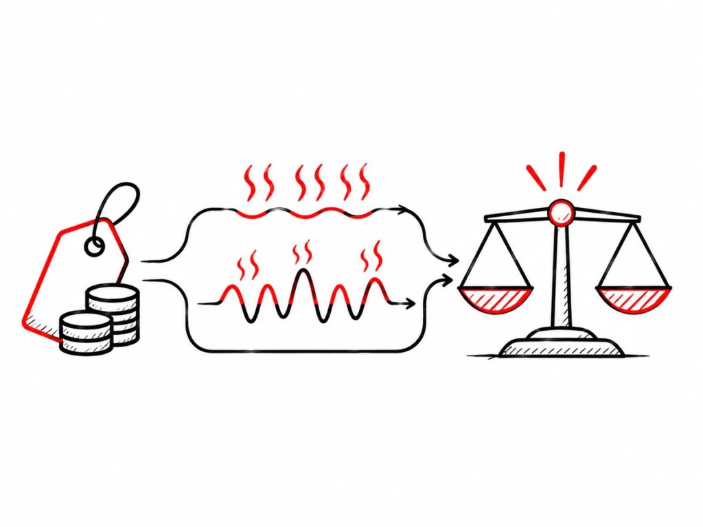
Three bids arrive for the same 75 kVA, 600 V to 208Y/120 V dry-type transformer. All three meet the federal efficiency minimum and carry the same certifications, and the spread between cheapest and most expensive is $1,500. The instinct is to award the low bid. But a dry-type transformer runs 8,760 hours a year for 25 to 30 years, and you bill its losses for every one of those hours — capitalized over a 20-year evaluation at ordinary commercial energy prices, every 100 W of core loss is worth roughly $1,100 in present-value dollars. The cheaper unit on the quote is often not the cheaper unit to own.
The tool that makes that visible is total cost of ownership, evaluated through the A and B factors utilities have used for decades and Canada’s dry-type efficiency standard recommends.
What Loss Evaluation Actually Measures
Transformer loss evaluation puts a present-day price on energy the transformer will waste in the future. It does not measure efficiency in the regulatory sense — a single percentage at a single test load — but the cost of losses across the actual operating life, at the actual loading, at the buyer’s actual energy price, discounted to present value. Two units with near-identical regulatory efficiency can carry very different lifetime loss costs if their losses are split differently between core and windings. Freight, duties and lead time sit outside the formula and deserve their own bid line.
The method comes from utility procurement, where it remains most common, and is formalized in IEEE C57.120-2017, which covers dry-type units and is currently under revision. The commercial and industrial buyer rarely asks for it: NEMA told the U.S. Department of Energy in 2017 that its low-voltage dry-type manufacturers seldom receive total-owning-cost requests. Most low-voltage dry-type transformers are still bought on price alone — exactly where loss evaluation tends to change the answer.
No-Load (Core) Losses vs. Load (Copper) Losses

The two loss components behave differently, which is why loss evaluation uses two factors. No-load loss is dissipated in the core whenever the transformer is energized, independent of load. Load loss is the I²R and stray loss in the windings and structural parts, scaling with the square of load current — at 50% load it dissipates 25% of rated load loss, at 30% only 9%.
That physics drives the economics: core loss is billed every hour of the year, so it carries the higher weighting per watt; load loss is weighted by how heavily and how long the unit is actually loaded. The reference conditions from how losses are measured matter: for dry-type regulatory testing, no-load loss is reported at 20°C and load loss corrected to 75°C. A bid quoting load loss at a different reference temperature, or a design value rather than a tested one, is not comparable without correction.
The A-Factor and B-Factor Formula, Explained
The standard loss-evaluation formula adds two capitalized loss terms to the purchase price:
Losses are entered in watts, load loss at rated load. A and B are dollars per watt — the present value of one watt of each loss type over the evaluation period — and they are specific to the buyer. A utility derives them from its energy cost, the capacity cost of serving losses at peak, and its financing rate, per the fuller C57.120 method. There is no universal A or B value, and any “standard” factor is somebody else’s assumptions.
For a commercial or industrial owner paying a blended energy rate, a simplified form is usually adequate — the annual cost of one watt running continuously, capitalized over the evaluation period:
B = A × (RMS per-unit load)²
The detail that trips people up is the RMS term. Because load loss follows current squared, the correct weighting is the average of the squared load, not the square of the average load. A unit loaded at 60% for 10 hours a day and 15% for the rest averages 34% but has an RMS load of 40%; squaring each (0.114 vs. 0.163), the average understates the load-loss cost by about 30%. Use interval metering where it exists; otherwise a load estimate from diversity factors is the honest fallback, provided the RMS correction is applied.
One limitation: the formula assumes sinusoidal current. On feeders dominated by drives, LED drivers or IT loads, harmonics raise winding eddy and stray loss above the rated figure — IEEE C57.110-2018 quantifies it — and ignoring this undervalues the load-loss term.
Where CSA C802.2 Ties Into This Math
The Canadian efficiency standard for dry-type transformers is built on this methodology: CAN/CSA-C802.2-18 recommends the total ownership cost methodology as the means of achieving its efficiency values, particularly for electric utilities, with a modified TOC method for other users. The standard’s own framing treats owner-specific loss evaluation as the way to decide how far above the efficiency floor a purchase should sit.
One wrinkle: for units manufactured from 2016 onward, the binding federal minimums are set directly in Canada’s Energy Efficiency Regulations, 2016 (SOR/2016-311), tested at 35% of nominal load for low-voltage units and 50% for medium-voltage — a specification calling for “CSA C802.2-12” is out of date — and the two countries’ efficiency rules diverge in April 2029. Neither regime prices the losses for you: a regulatory minimum says a unit is legal to sell; only a loss evaluation says whether it is economical to own.
Running a Transformer TCO Calculation Step by Step

The worked example uses the opening’s three bids. Every price, rate and loss figure is illustrative — plausible for a 75 kVA general-purpose isolation transformer in a Canadian commercial building, not official rates or published product values.
Step 1: Set the economic inputs. Assume $0.12/kWh blended energy, a 7% discount rate, and a 20-year evaluation period. The present-worth factor is [1 − 1.07−20] ÷ 0.07 = 10.59, so the A-factor is 0.12 × 8,760 ÷ 1,000 × 10.59 = $11.14 per watt of no-load loss.
Step 2: Set the loading. Assume an RMS load of 45% of nameplate. The B-factor is 11.14 × 0.45² = $2.26 per watt of rated load loss.
Step 3: Collect tested losses from each bid. Bid X is $6,800 with 200 W no-load and 1,400 W load loss. Bid Y is $8,300 with 150 W and 1,250 W. Bid Z is $7,400 with 240 W and 1,050 W. All three land between 98.6% and 98.9% at the 35% regulatory test point, so efficiency alone does not separate them.
Step 4: Capitalize and add. Bid X: 6,800 + (11.14 × 200) + (2.26 × 1,400) = $12,184. Bid Z: 7,400 + 2,673 + 2,368 = $12,441. Bid Y: 8,300 + 1,670 + 2,819 = $12,789.
At 45% loading, the low bid wins on its merits — loss evaluation exists to confirm that as much as to overturn it. The premium unit, Bid Y, has the lowest losses and still loses: its $1,500 premium buys about $900 of present-value loss savings at these factors. Paying for efficiency is only worth it when the factors say so — the efficiency features worth paying for depend on the installation, not the catalogue.
Now change one input. At 30% RMS loading, B falls to $1.00 per watt and Bid X extends its lead, $10,430 against $11,125 for Z. At 65%, B rises to $4.71, load loss dominates, and Bid Z takes over at $15,013 against $15,614 for X. The ranking flips on the loading assumption alone: a low-core-loss design rewards lightly loaded transformers, a low-winding-loss design rewards heavily loaded ones, and no single unit is the efficient choice everywhere.
The loss figures in Step 3 must be tested values at the same reference temperatures, ideally backed by the factory testing that verifies them: overstating Bid Z’s load loss by 10% adds about $240 — roughly the margin separating it from Bid X.
Where to Run the Numbers on Your Own Transformer
The quickest way to test a real bid comparison is Rex’s transformer savings and payback calculator: enter the losses and price of two transformers, an energy price and a loading level, and it returns each unit’s annual loss cost and the payback of the lower-loss option at 8,760 energized hours per year. Its output is undiscounted — multiply the annual difference by the Step 1 present-worth factor to compare with the A/B method.
It inherits the formula’s limits — no temperature correction, no harmonic allowance. For a quick screen of two quotes, that is enough; for a large order, a nonlinear load profile or a utility-style evaluation with demand charges, the full C57.120 method is the better basis.
The same comparison works against the transformer already in service: enter its tested losses with a price of zero, or the quoted repair cost, and the result is a first pass at when replacement beats repair. For an older unit, energy alone often does not justify the swap — worth knowing before the budget request goes in.
Conclusion
Transformer total cost of ownership comes down to one trade-off: lower losses cost money up front and save money every hour afterwards, and whether the saving outweighs the premium depends on the owner’s energy price, the discount rate, and above all the RMS loading of the unit. Core loss is paid in full regardless of load; winding loss scales with the square of it.
Wherever a few hundred watts of loss are at stake, require tested no-load and load losses at stated reference temperatures in every bid, and award on total evaluated cost rather than price. Derive A and B from your own energy price and a measured or properly RMS-corrected load profile, never from a borrowed factor. If the low bid still wins, buy it with confidence. If it doesn’t, the evaluation has just paid for itself.